⚖️ The Equilibrium and its Fluctuations

Economic Fluctuations

Time Horizons

• Short Run (SR): < 2-3 years. Prices are often sticky.
• Medium Run (MR): 5-8 years.
• Long Run (LR): 10-30 years.

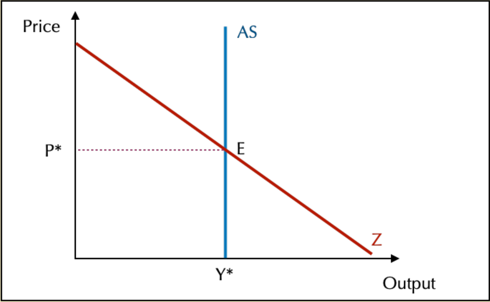
Aggregate Demand and Supply

We analyze the equilibrium using Aggregate Demand (AD) and Aggregate Supply (AS).

Aggregate Demand (AD)

It represents the total demand for goods and services in the economy.

$$AD=C+I+G+(X-M)$$

The AD curve is downward sloping: as the price level ($P$) decreases, demand increases.

Aggregate Supply (AS)

It represents the total quantity of goods and services that firms produce and sell.

• Short Run AS: Upward sloping (or horizontal in extreme Keynesian view).
• Long Run AS: Vertical (determined by factors of production, independent of price).

Elasticity

Definition

Elasticity measures the responsiveness of one variable to changes in another.

Price Elasticity of Demand: How much the quantity demanded changes when the price changes.

• Elastic: Quantity changes a lot (e.g., luxury goods).
• Inelastic: Quantity changes little (e.g., gasoline, necessities).

If the price of gasoline skyrockets, demand might not drop immediately (inelastic in the short run) because people still need to drive to work. But over time, they might buy electric cars (more elastic in the long run).

Elasticity for Demand (Price Elasticity)

🇫🇷 Élasticité prix

Since the quantities adapts to the prices levels, we will look on prices variations. If the demand dose not move that much after a price change, the product is said inelastic. On the opposite, it will be called elastic. This means that the demand's courbe will not have the same shape depending on psychological/sociological/tensions on consumers. Some pasterns are recognizable:

• Close substitues (bien plutôt substituables), if you can switch from apples to pears (Competition) -> very elastic.
• Necessity goods (bien de 1ère nécessité) -> inelastic.
• Time horizon (horizon temporel) -> elasticity rise with times, as individuals adapt their habits.

Here is the example of graphs, with inelastic/elastic goods:

Memory Tip

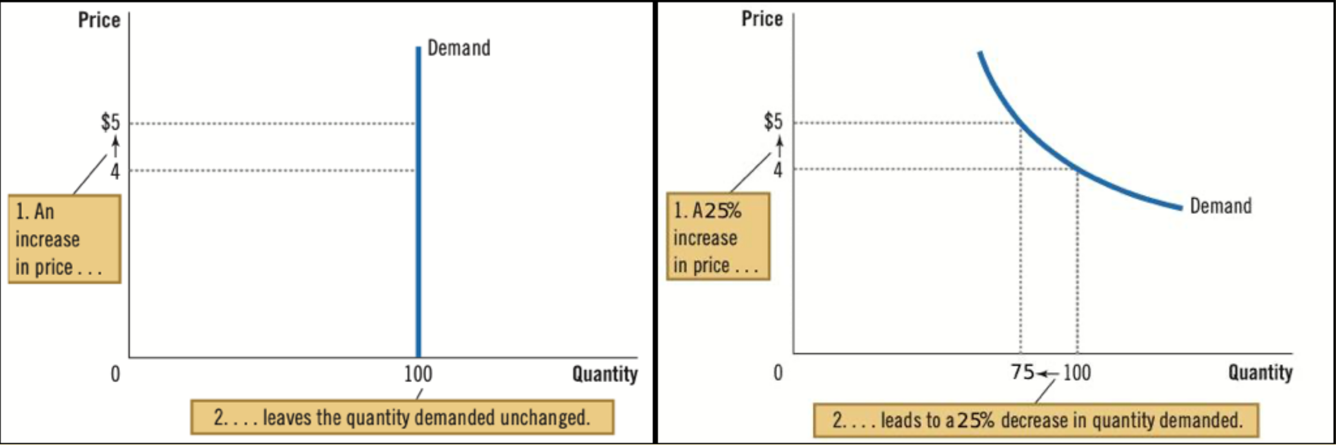
The demand curve for inelastic goods looks like an I, like Inelastic!

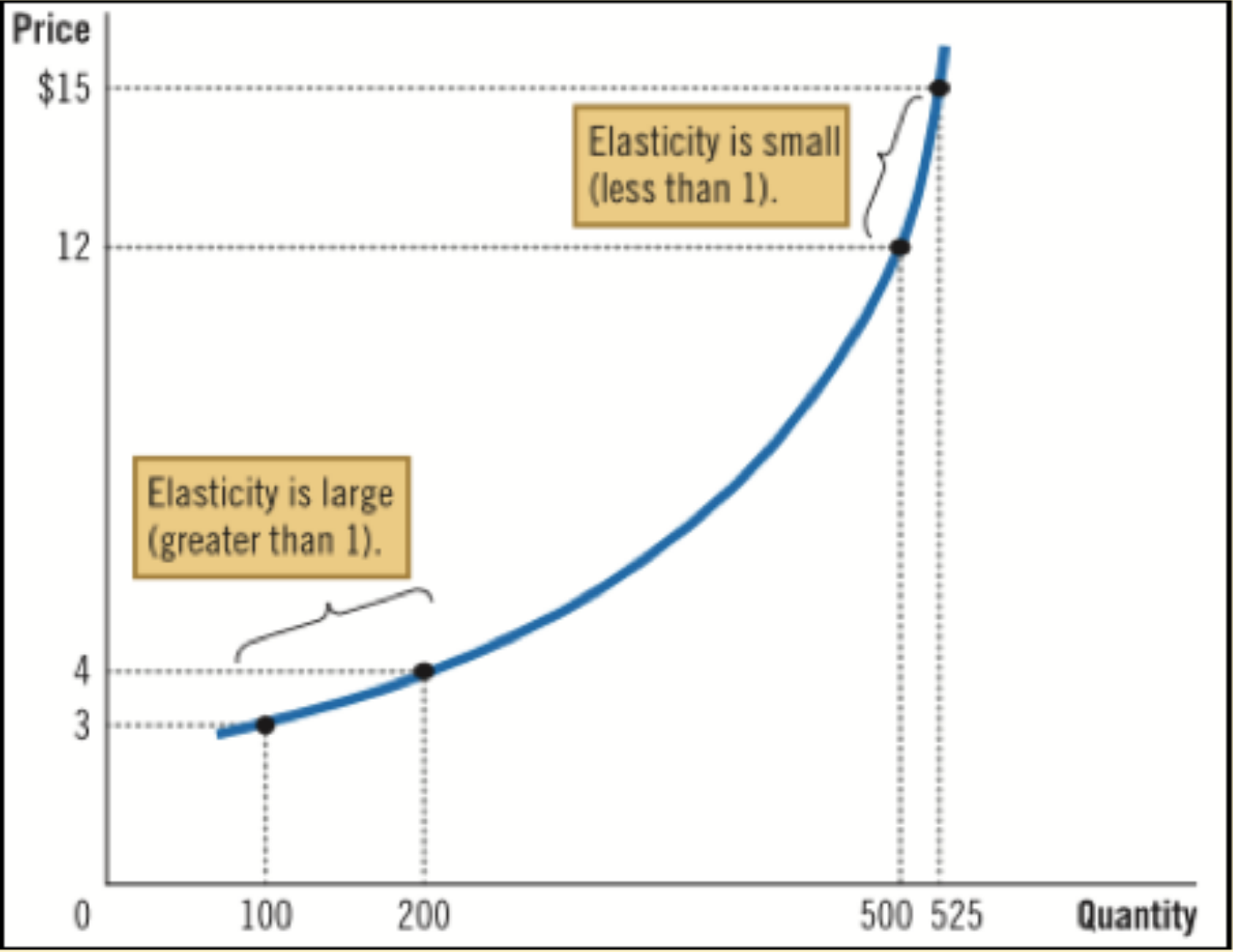
For the flowing curves, here is the elasticity factor:

1. ${ϵ}_p(d)=\frac{\mathrm{\Delta }Q/Q}{\mathrm{\Delta }P/P}=\frac{50/100}{1/4}=2$
2. $ϵ=\frac{\mathrm{\Delta }Q/Q}{\mathrm{\Delta }P/P}=\frac{25/100}{1/4}=1$ When the proportion of quantity moves more over price, the elasticity is > 1. If's it a perfect 1, then it's a perfect (unit) elasticity. The flatter the curve is at a given point, the greater the elasticity will be. The steeper the curve is, the less elastic the demand/supply will be.

Elasticity of supply

It's the same rules as above, but with a different symbol. More quantity you bought, less impact the price change will have on you. Opposite for small quantities.

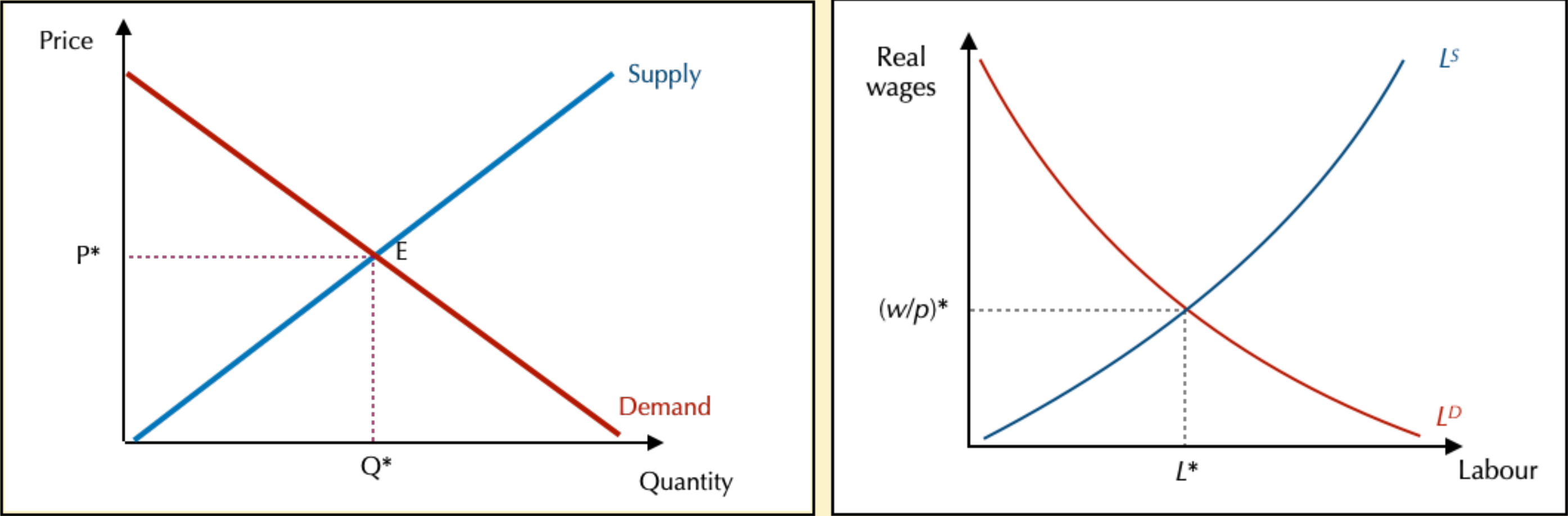
The curve is inelastic at the start as even with not so many workers, they will prefer to use capital and so not be impacted that much. At the opposite, if the cost of labour decrease, they will use it even more, to spend even less capital.

Sale thing for the worker; if you are rich, being a bit more rich isn't that much. But if you're poor, then even a little change could make a lot.

On the goods & services market, a lot of substitutions are possible, and so a lot of elasticity is possible everywhere,

Document 8 (Correction)

A tax on production (Corporate Income Tax) means that corporations will have to sell less, as demand is lower (as price is higher) and so will resolve to less work force & capital and so, at the end, in a decrease of worker's salary/licensing. But if the equilibrium salary decrease, then the number of workers did. With the graphs, more workers where working in the first place, more the hit from the decrease of the labor needed will be HUGE.

A cut in the corporate tax would be a good idea — according to our graphs — but it doesn't mean it will work for sure. The benefits could be invested in Capital and not Work Forces, or not invested at all. If we take a look at the graphs we built earlier, if the demand is more impacted that the supply, then corporate owners win more than workers.

Perte de surplus

La taxe impacte une perte de surplus des producteurs et des consommateurs (voir le cours précédent). Plus l'offre est élastique, la perte sèche (du surplus) est plus élevé. Si elle est inélastique, la perte est moindre (car le producteur prend cher) 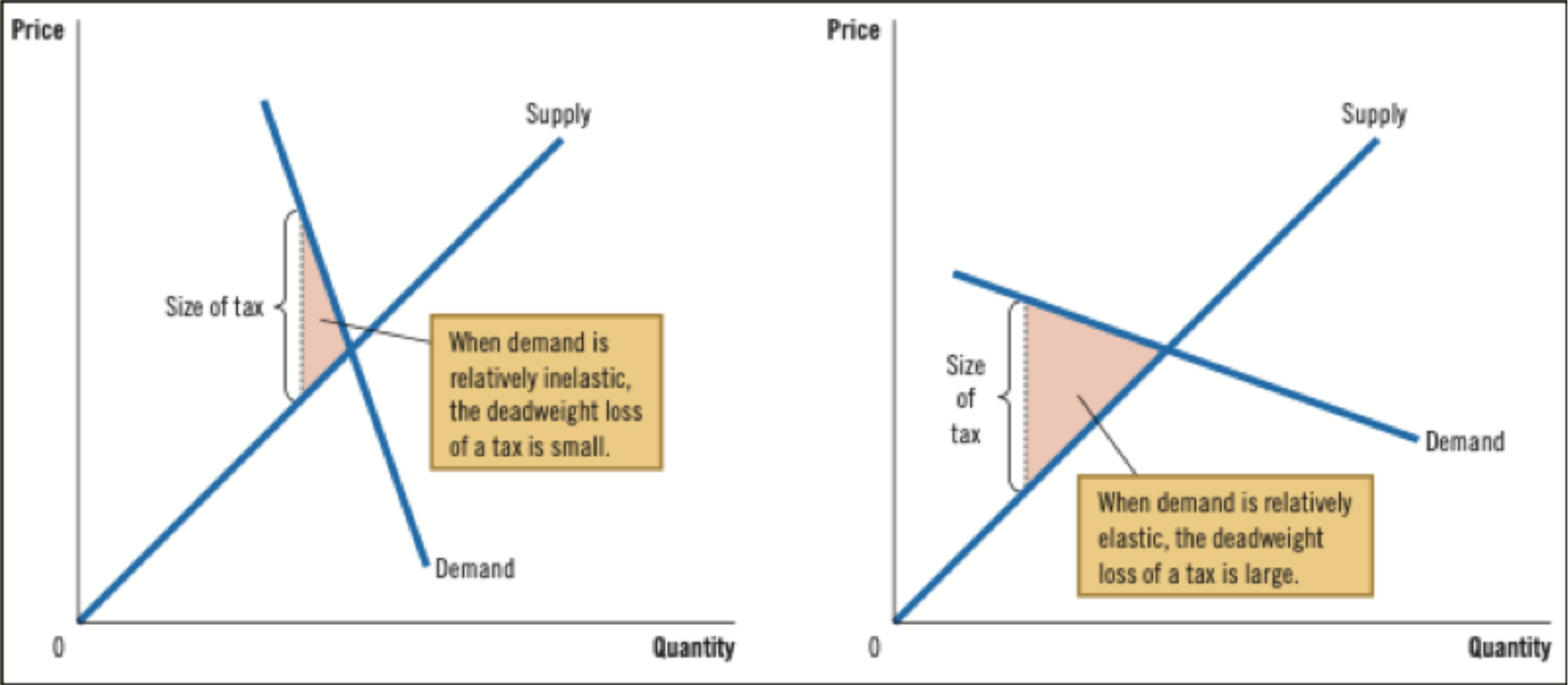(here, the variations are on the curb of demand)

Global trends on growth and unemployment

Growth over time

General tendances to keep in mind.

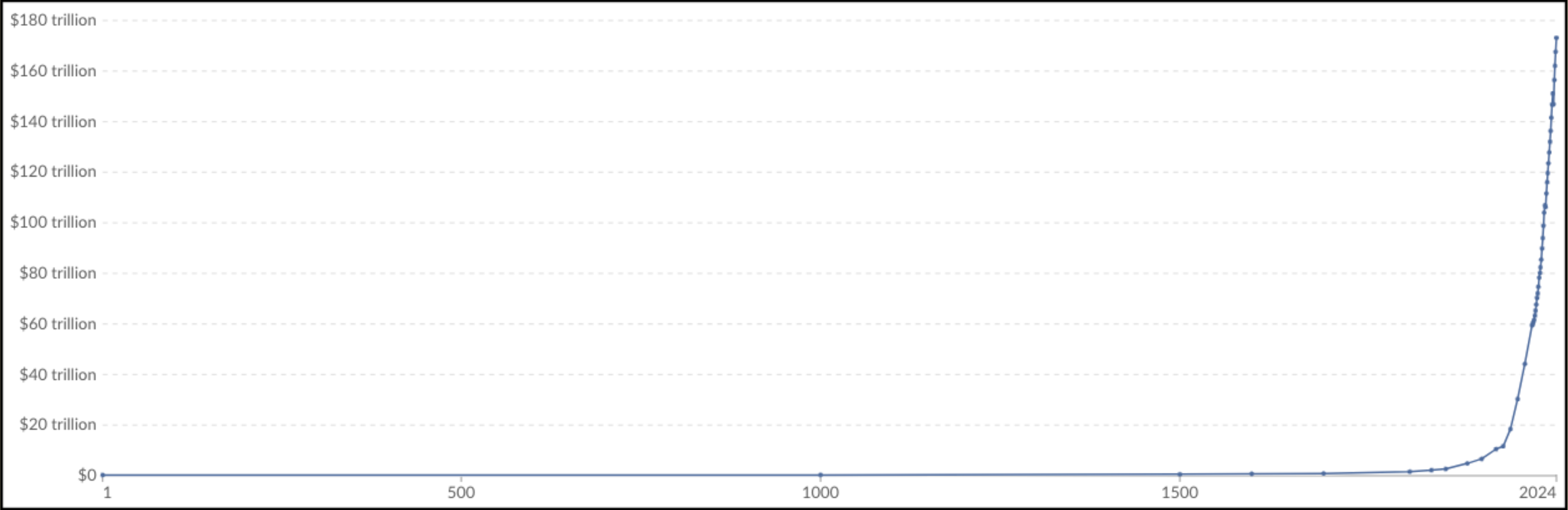Growth is a quite recent phenomenal. And it is exponential. The first effects on growth by the industrial evolution is 1820.

But if we take a closer look...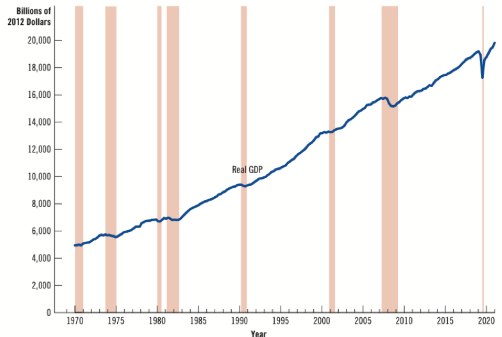

SOMETIME THE GDP DECREASES ! And guess what: it always match with crises:

• 1970: first oil crises with war in middle east
• 1974: second one
• 1980: third one
• 2001: internet bulle
• 2007: sub primes
• 2019: Covid (my beloved)

This growth in unstable. We analyse growth over time. We need an increase on the long term (and so we look around on the long term).

Smith starts to look on growth ~ so it's a long time economics object.

Economists will not look at the nominal GDP but as the real GDP which take accounting of the inflation.

Measuring the cost of living

How could we mesure the cost of living? We note $CPI$, (IPC, indice du prix à la consommation) a mesure of how much goods types are bought by a "typical consumer" and more importantly the evolution over time, and the impact of inflation. Here is an example on how it could goes :

1. We create a basket (2 hamburger and 4 hot-dogs)
2. We make survey around the country to check the price
3. We make a small little juicy delta to see how much it evolved

$$\text{Real GDP}=\frac{\text{Nominal GDP}}{\text{CPI}}$$

Real GDP will so decrease if CPI increase of Nominal PIB decrease (like any fractions).

What link between growth and unemployment?

Warning

For all of this chapter, keeps in mind that it's neoclassical and so deeply politically engaged. They stands for No-State-Intervention

Before computing this rate, we need to understand what is an unemployed person. You need to:

• Look for a job
• Be registered at a public unemployment service
• Be available to work within a month

If you are not looking for a job, you are an unactive person. This include:

• retired
• underage
• poeple that never worked
• not interest in work (c.f. voluntary unemployment)

Actives people have a job. Sometimes, people can be in-between, like if you are on a partial time and looks for a full time job.

Actives and inactives are what we call the labor force of a country. This way, the Unemployment rate is computed as it: $$U = \frac{\text{Number of active unemployed}}{\text{Labour Force}} \times 100$$ The participation rate is compute as followed: $$\frac{\text{actives}}{\text{people that can work}}$$ This way, we can know how much people are involved in the labor market, and how much of them are unemployed and looking for a job.

You have a negative (~ opposite) implication between GDP and $U_{\text{Rate}}$. If you want to produce more, you need more work force, and so reduce the unemployed rate.